TravelingPacket – A blog of network musings

When deploying wireless networks one of the best practices is to limit the SSIDs used within the WLAN. The reason we want to limit the amount of SSIDs, is the SSID announcement is sent through a Beacon frame. This frame is a broadcast to all stations. This happens every 100 MS or 102.4 MS according to how busy the medium is. In all documentation and great blogs I have not found a lot of visual examples of what actually happens, So I thought this might be a cool blog entry to write.

On top of the constant beacon broadcasting of the APs, when a client wants to join, it will send a probe request to the broadcast address of ff:ff:ff:ff:ff:ff and all APs will respond with a probe response frame directly to the station informing the client of the SSID and its supported capabilities. Beacons and probe request/response frames are the reason we need to limit the amount of SSIDs. For instance (and I will show this below) if you had 1 AP with 5 SSIDs, with 1 client trying to connect, the AP would be sending somewhere around 50 Beacons in 1 seconds, and 5 probe responses. This is might not seem like a lot of air time used at first, but think if you had 5 clients trying to connect at the same time, or maybe 2 or more APs on the same channel, with 5 clients trying to connect at the same time. Then the airtime usage goes up huge. Since wireless is half-duplex this takes increases the time it takes for clients to do what they need to do on the spectrum.

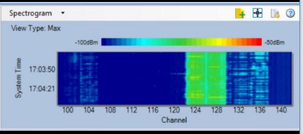
To show the results, I am using the Ekahua sidekick with spectrum analysis. I will start with 1 AP broadcasting 1 ssid, and then add another AP on the same channel. From there I will increase the SSIDs and show the airtime usage.  I hope to show why it is important to keep SSID overhead to a minimum. The gear used will be a Ruckus Zondirector, Ruckus 7982, and R710 APs. I am lucky enough to have an area with very little neighboring wifi networks, so I am testing with 1 wireless client in range of the AP to limit, and show the probe request/response traffic. I am broadcasting the test SSIDs on channel 11 and channel 157.

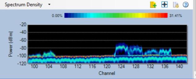
First lets look at just 1 AP with one SSID broadcasting.

As you can see from above, very little spectrum usage. Again, no clients are connected to an SSID, and only one device would be doing probe requests.

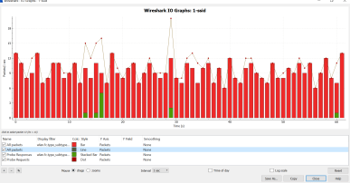
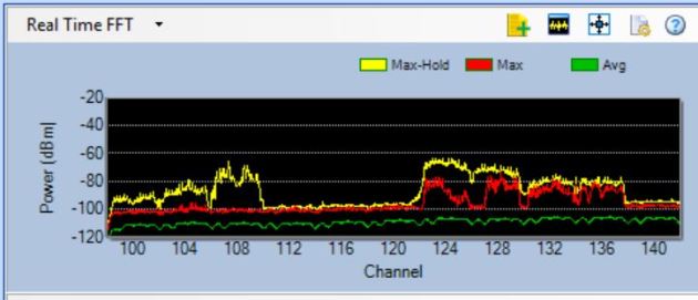
I did a packet capture next, check out the analysis data and the size of the capture. I only let the capture run for 1 minute (60 seconds). The size of the file was roughly 165 Kb. The red in the graph below represents beacon frames, and the dots/green are probe requests vs probe responses.

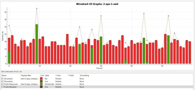
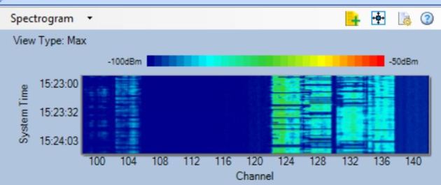
I then added the other AP on the exact same channels, still only broadcasting 1 SSID. Spectrum usage definitely increased but only by very little. Below are the spectrum density graphs and Wireshark IO graph.

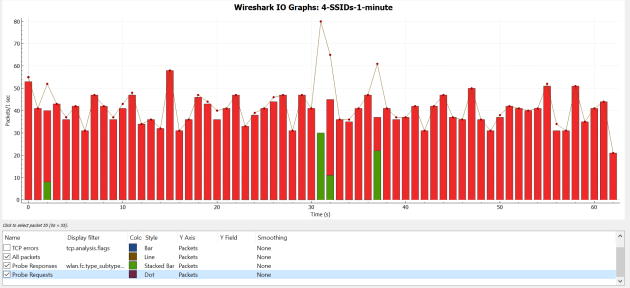
Now, lets increase things a bit – I will start broadcasting 4 SSIDs from 1 AP.

Spectrum usage from 1 AP broadcasting 4 SSIDs:

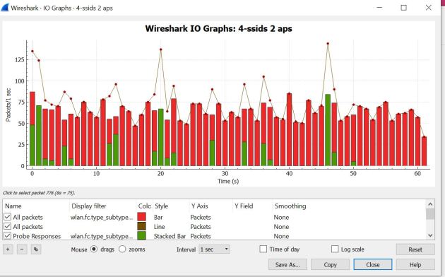
Below is 2 APs broadcasting 4 SSIDs – all on the same channels.

When comparing the wireshark IO graph we can really see how many Beacon frames are sent and compare those between 1 and 2 APs. Another cool thing to note is the size of the wireless PCAPs – each running for 1 minute, the 1 AP broadcasting 4 SSIDs size was 662 KB, and 2 APs broadcasting 4 SSIDs each was just about double at 1200 KB. In the graphs below, red indicates the number of Beacon frames.

2 APs – 4 SSIDs:

After all the testing, we have a big increase from just adding 1 SSID and an even bigger increase from having another AP broadcasting on the same channels. This isn’t ground breaking but cool to see in action. I have seen many many clients have at least 6 SSIDs broadcasting, and this give some good illustration on why we need to reduce the amount of SSIDs in use. There are a few tools out to calculate the SSID overhead – tools such as http://www.revolutionwifi.net.

Check out the below picture comparing 1 SSID to 4 SSIDs just from 1 AP for 2.4 and 5 gig.

1AP 1-SSID

1 AP 4-SSIDs

1 AP 1 SSID

1 AP 4 SSIDs

.

One great way to troubleshoot wireless issues that clients might be having is to perform a packet capture or use some kind of wireless analysis tool. In this case I have an Ekahau sidekick with Capture. Before this tool I used Ubuntu, Wireshark, and a compatible wireless adapter to capture packets. The MCS or Modulation and Coding Scheme value indicates a lot about the client. For example, the MCS rate is as really a reference number given to the combination of  – amount of Spatial streams, Modulation type and coding scheme. Analyzing the MCS helps when we need to troubleshoot the common problem of “its slow” while everything looks good.

I look at the MCS rate when troubleshooting client problems for a lot of reasons. Since the MCS rate is a reference number describing how much data can be sent over the wireless medium, it gives us an idea of the wireless environment. If the spectrum has lots of contention/interference or the client has low RSSI then the MCS will reflect this. If clients have lots of retrys, or a low RSSI then it will lower the modulation scheme, and therefore lower the MCS rate.

Lets take a look at a 802.11ac packet in Wireshark and break down what each section means. The MCS is located in the Data frame under the 802.11 Radio information section.

This packet is captured from a Data frame, you will notice the MCS rates are only captured on data packets – Lots of reasons for this. Most management/control frames are sent with the lowest data rate possible to allow them to be understood by clients far away, or if the network is very congested.

In this example we are looking at an 802.11ac frame, and we see right away the MCS index is 7  – from looking at the MCS chart we see that means modulation:64 QAM, which a number 5/6 . The 5/6 is the actual FEC or Forward error correction coding rate, which is given in fraction form. 5/6 equals to 0.83333.. which means that 83% of the data stream can be used to send real data. 5/6 is the highest coding rate.

We can see that the host has 2 Spatial streams, is using a Short guard interval , 40 MHz channel and the data rate is 300 – the data rate is  the highest capable with these settings. Notice the RSSI is -44 and we are just using 64 QAM, you really have to be close and have a clear spectrum to achieve 256 QAM.

Below  is the table of MCS rates for 802.11AC/N – Compliments of WLANPROS.com

Inter frame spacing is some of the magic in WiFI. Its also one of the more confusing aspects of studying and understanding how WMM, and processes like Point coordination function work. Inter frame spacing is used to help avoid collisions on the wireless spectrum.

When a station wants to send a frame there are two methods that have to be OK before it can do this. 1 – Physical Carrier sense. Physical Carrier Sense is the process of checking to see if the wireless medium is busy. It does this my checking the wireless medium for RF energy, if it is above a certain threshold then it will wait to send.

The second check is Virtual Carrier sense. This method looks at passing wireless frames and sets a local MAC layer timer called the Network allocation vector or NAV to the amount of time found in the passing frame’s Duration field. When this reaches 0 it attempt a Physical Carrier sense. If the NAV is 0 and Physical Carrier sense shows RF energy below its threshold – the station will then wait the length of a Interframe space, then wait through the random backoff algorithm time (decided by the contention window), run through the carrier sense process again – then will actually send the frame.

The importance of the IFS is that the station has to wait that given amount of time. In the section below all the different IFS are listed with the its length of time. When studying for the CWAP exam I had a hard time remembering them, so hence the blog entry.

Once the station has the okay to send (Carrier sense is good) then it will wait the given IFS length. This is a big deal because not only does the STA wait the length of time before attempting to send the frame, but it can be used to give priority to certain frames over others. We do this by having that station wait less time then others based on the type of frame they are sending. By Priority I mean it asks the client to wait a smaller amount of time before sending the packet with a higher priority – This is called Probabilistic priority.

The following is a quick list of interframe spacing methods and are ordered by the duration time – shortest to longest time.

RIFS – Reduced IFS – Shorter than SIFS. Came out in 802.11n , to help minimize overhead. RIFS are used when one transmitter is sending packets when no SIFS reponses are expected. This IFS is not used in 802.11ac.

SIFS – Short Interframe Spacing – Shortest of all IFs . Used for ACKs, CTS in response to RTS, and the first data frame following the CTS.

PIFS – Point Coordination interframe space. – Used by the Point Coordination function to gain access to the medium. Used when switching from Distributed Coordination to Point Coordination

DIFS – DCF (Distribution coordination function) Interframe spacing– used with normal data frames. After the completion of sending a data frame the duration of a DIFS must be waited before attempting to send another.

AIFS – Arbitration IFS – Used in a kind of QoS manner. When a QoS station send data frames it waits an AIFS. Also used on a few control frames such as PS-Poll, CTS when not responding to a RTS (Thats a SIFS), BlockACKs, and RTS frames. A neat thing abou the AIFS is that the time is configurable on the AP, and then transmitted to clients by the Beacon frame.

EIFS – Extended IFS – Extended for a reason – When a frame is received with errors or corrupted the receiver will respond with  EIFS which tells the sender to wait for a longer period so it can see if the packet was delivered correctly. Once this happens, it will start go back to using a normal DIFS or AIFS .

Inter frame spacing gives us another mechanism to help avoid collisions in 802.11. It does this by having the Station wait a given amount of time (IFS) according to the type frame being sent.  We do this by utilizing Carrier sense, random back off timer, IFS and contention windows.

Spectrum analysis in 802.11 design is extremely important. Detecting which channels are in use in 2.4 and 5 gig spectrum’s as well as the channel density is a great help when channel planning or troubleshooting wifi issues. There are lots of graphs within any spectrum analyzing software.  Below are a few that I feel really help narrow down issues within spectrum.

FFT Graphs

FFT stands for Fast Fourier Transform – Which is an algorithm that samples signals over a period of time. One of the most usable graphs when looking at the spectrum is the FFT density graph and the real time FFT graph. I am currently using Fluke’s or now NetScouts SpectrumXT.

The below images shows the FFT of our office. As you can easily see just from the FFT graphs that channel 124 and 128 is heavily in use. This is because of a few reason – 1 we are using 40 MHZ channels so channel 124 and 128 are combined.  2 – the AP using these channels are the closest to me, the other APs are pretty far away.

So why is this important during a survey or just checking to see whats going on – its important because it shows the amount of energy used on those channels. An abundance of energy will cause slowness and clients to defer sending as well as packet loss. Understanding and viewing spectrum is also extremely important in channel selection and design.

So lets compare the above with the Real time FFT – the Real time graph changes as the name states very often. But the Density and Real Time should be pretty similar. For channel planning purposes you can easily recognize that channels 124 through 136 should not be used. Lots of channels are open and can be used in this range that will not cause any interference.

Spectrogram

The next graph is the famous Spectrogram. The Spectrogram graph shows the amplitude of a signal over time. Basically it shows how busy and strong the signals are on that channel. These are also know as sweep or waterfall graphs. This graph shows how much signal density is on that channel. For example, if you have a channel maybe 104 that has traffic on it (seen by FFT), but its usage is very low (Spectrogram) then we know that that channel even though used would have very low interference, where as Channel 124 has lots of traffic and usage.

In the following graph the darker color shows more usage, notice Channel 124 which my STA is on.

.

The following graph shows the spectrum after my station starts downloading a huge file on WIFI. Check out the difference in usage.

There are a lot of spectrum analysis graphs some are very helpful. These are two graphs that I find that help a lot to pinpoint the usage and channel use/layout of a wireless network. There are many more helpful graphs such as the wifi integrated graphs that can collect retries, Channel SNR, etc.